miércoles, 10 de febrero de 2010
Solid state (electronics)
Solid-state electronics are those circuits or devices built entirely from solid materials and in which the electrons, or other charge carriers, are confined entirely within the solid material. The term is often used to contrast with the earlier technologies of vacuum and gas-discharge tube devices and it is also conventional to exclude electro-mechanical devices (relays, switches and other devices with moving parts) from the term solid state. While solid-state can include crystalline, polycrystalline and amorphous solids and refer to electrical conductors, insulators and semiconductors, the building material is most often crystalline semiconductor. Common solid-state devices include transistors, microprocessor chips, and DRAM. A considerable amount of electromagnetic and quantum-mechanical action takes place within the device. The expression became prevalent in the 1950s and the 1960s, during the transition from vacuum tube technology to semiconductor diodes and transistors. More recently, the integrated circuit (IC), the light-emitting diode (LED), and the liquid-crystal display (LCD) have evolved as further examples of solid-state devices.
In a solid-state component, the current is confined to solid elements and compounds engineered specifically to switch and amplify it. Current flow can be understood in two forms: as negatively-charged electrons, and as positively-charged electron deficiencies called electron holes or just "holes". In some semiconductors, the current consists mostly of electrons; in other semiconductors, it consists mostly of "holes". Both the electron and the hole are called charge carriers.
For data storage, solid-state devices are much faster and more reliable but are usually more expensive. Although solid-state costs continually drop, disks, tapes, and optical disks also continue to improve their cost/performance ratio.
The first solid-state device was the "cat's whisker" detector, first used in 1930s radio receivers. A whisker-like wire was moved around on a solid crystal (such as a germanium crystal) in order to detect a radio signal.[6] The solid-state device came into its own with the invention of the transistor in 1947.
Examples of non-solid-state electronic components are vacuum tubes and cathode-ray tubes (CRTs).
---
Teone Salazar
Comunicaciones de Radio Frecuencia
http://en.wikipedia.org/wiki/Solid_state_%28electronics%29
Circulators and isolators
Why are circulators and isolators relatively expensive in the world of cheap microelectronics? Because for the most part they are hand assembled, tuned and tested. Tolerances on material properties of the ferrite and magnet as well as mechanical tolerances mean that invariably someone must make at least minimum wage tweaking the product. Tuning methods are different at different manufacturers. One method is to design the part so that the ports are all greater than 50 ohms, then tweak the impedance down by squeezing RTV over the traces to increase their capacitance while watching the result in real time on a network analyzer.
Circulators
A circulator is a ferrite device (ferrite is a class of materials with strange magnetic properties) with usually three ports. The beautiful thing about circulators is that they are non-reciprocal. That is, energy into port 1 predominantly exits port 2, energy into port 2 exits port 3, and energy into port 3 exits port 1. In a reciprocal device the same fraction of energy that flows from port 1 to port 2 would occur to energy flowing the opposite direction, from port 2 to port 1.The selection of ports is arbitrary, and circulators can be made to "circulate" either clockwise (CW) or counterclockwise (CCW).
A circulator is sometimes called a "duplexer", meaning that is duplexes two signals into one channel (e.g. transmit and receive into an antenna). This is not to be confused with the term "diplexer" which is refers to a filter arrangement where two frequency bands are separated into two channels from a single three-terminal device. A lot of people mix up these terms. You can remember the correct definitions because "filter" and "diplexer" both have an "i" in them, and "circulator" and "duplexer" both have a "u".
What are circulators good for? The make a great antenna interface for a transmit/receive system. Energy can be made to flow from the transmitter (port 1) to the antenna (port 2) during transmit, and from the antenna (port 2) to the receiver (port 3) during receive. Circulators have low electrical losses and can be made to handle huge powers, well into kilowatts. They usually operate over no more than an octave bandwidth, and are purely an RF component (they don't work at DC).
Circulator rule of thumb!
Isolators
By terminating one port, a circulator becomes an isolator, which has the property that energy flows on one direction only. This is an extremely useful device for "isolating" components in a chain, so that bad VSWRs don't contribute to gain ripple.Circulators and isolators can be made from 100's of MHz to through W-band (110 GHz). They can be packaged as planar microstrip components, coaxial components or as waveguide components. Waveguide circulators and isolators have by far the best electrical characteristics. You can specify insertion loss down to less than 0.2 dB in some cases! Microstrip and coax circulators and isolators might have losses between 0.5 and 1.0 dB. Note that the more bandwidth you ask for, the crummier the insertion loss and isolation will be.
Circulator vendors
There are probably 100 garage shops around the country that claim to be circulator manufacturers, be careful who you buy from. There are many reputable circulator vendors for circulators. But from now on, we are NOT going to give them any free advertising! If you want some advice on which vendors to look at, contact us by email and we'll help you out. Better still, tell your favorite circulator vendor to get in touch with us to sponsor this page!Switchable circulators
A really cool type of circulator is a switchable circulator, in which an electrical signal is used to switch the orientation of the circulator from CW to CCW and vice versa. The way the circulator is constructed it latches into a particular orientation and will stay there in the absence of the electrical signal, say, for instance your power supply goes off. The means for switching the orientation is a single high-current DC pulse that is provided by the driver circuit. This in an expensive technology, but it makes an unbelievably low-loss RF switch with high power handling.--
Teone Salazar
Comunicaciones de Radio Frecuencia
http://www.microwaves101.com/encyclopedia/circulators.cfm
Cavity Magnetrons
Cavity magnetron
The cavity magnetron is a high-powered vacuum tube that generates microwaves using the interaction of a stream of electrons with a magnetic field. The 'resonant' cavity magnetron variant of the earlier magnetron tube was invented by Randall and Boot in 1940.[1] The high power of pulses from the cavity magnetron made centimetre-band radar practical. Shorter wavelength radars allowed detection of smaller objects. The compact cavity magnetron tube drastically reduced the size of radar sets[2] so that they could be installed in anti-submarine aircraft[3] and escort ships.[2] At present, cavity magnetrons are commonly used in microwave ovens and in various radar applications.[4]Construction and operation

A similar magnetron with a different section removed (magnet is not shown).

The magnetron is a self-oscillating device requiring no external elements other than a power supply. A well-defined threshold anode voltage must be applied before oscillation will build up; this voltage is a function of the dimensions of the resonant cavity, and the applied magnetic field. In pulsed applications there is a delay of several cycles before the oscillator achieves full peak power, and the build-up of anode voltage must be coordinated with the build-up of oscillator output. [5]
The magnetron is a fairly efficient device. In a microwave oven, for instance, a 1.1 kilowatt input will generally create about 700 watt of microwave power, an efficiency of around 65%. (The high-voltage and the properties of the cathode determine the power of a magnetron.) Large S-band magnetrons can produce up to 2.5 megawatts peak power with an average power of 3.75 kW.[5] Large magnetrons can be water cooled. The magnetron remains in widespread use in roles which require high power, but where precise frequency control is unimportant.
Applications

Radar
In radar devices the waveguide is connected to an antenna. The magnetron is operated with very short pulses of applied voltage, resulting in a short pulse of high power microwave energy being radiated. As in all radar systems, the radiation reflected off a target is analyzed to produce a radar map on a screen.Several characteristics of the magnetron's power output conspire to make radar use of the device somewhat problematic. The first of these factors is the magnetron's inherent instability in its transmitter frequency. This instability is noted not only as a frequency shift from one pulse to the next, but also a frequency shift within an individual transmitter pulse. The second factor is that the energy of the transmitted pulse is spread over a wide frequency spectrum, which makes necessary its receiver to have a corresponding wide selectivity. This wide selectivity permits ambient electrical noise to be accepted into the receiver, thus obscuring somewhat the received radar echoes, thereby reducing overall radar performance. The third factor, depending on application, is the radiation hazard caused by the use of high power electromagnetic radiation. In some applications, for example a marine radar mounted on a recreational vessel, a radar with a magnetron output of 2 to 4 kilowatts is often found mounted very near an area occupied by crew or passengers. In practical use, these factors have been overcome, or merely accepted, and there are today thousands of magnetron aviation and marine radar units in service. Recent advances in aviation weather avoidance radar and in marine radar have successfully implemented solid-state transmitters that eliminate the magnetron entirely.
Heating
In microwave ovens the waveguide leads to a radio frequency-transparent port into the cooking chamber.Lighting
In microwave-excited lighting systems, such as a sulfur lamp, a magnetron provides the microwave field that is passed through a waveguide to the lighting cavity containing the light-emitting substance (e.g., sulfur, metal halides, etc.)History
The first simple, two-pole magnetron was developed in 1920 by Albert Hull[6] at General Electric's Research Laboratories (Schenectady, New York), as an outgrowth of his work on the magnetic control of vacuum tubes in an attempt to work around the patents held by Lee De Forest on electrostatic control.Hull's magnetron was not originally intended to generate VHF (very-high-frequency) electromagnetic waves. However, in 1924, Czech physicist August Žáček[7] (1886-1961) and German physicist Erich Habann[8] (1892-1968) independently discovered that the magnetron could generate waves of 100 megahertz to 1 gigahertz. Žáček, a professor at Prague's Charles University, published first; however, he published in a journal with a small circulation and thus attracted little attention.[9] Habann, a student at the University of Jena, investigated the magnetron for his doctoral dissertation of 1924.[10] Throughout the 1920s, Hull and other researchers around the world worked to develop the magnetron.[11][12][13] Most of these early magnetrons were glass vacuum tubes with multiple anodes. However, the two-pole magnetron, also known as a split-anode magnetron, had relatively low efficiency. The cavity version (properly referred to as a resonant-cavity magnetron) proved to be far more useful.
While radar was being developed during World War II, there arose an urgent need for a high-power microwave generator that worked at shorter wavelengths (around 10 cm (3 GHz)) rather than the 150 cm (200 MHz) that was available from tube-based generators of the time. It was known that a multi-cavity resonant magnetron had been developed and patented in 1935 by Hans Hollmann in Berlin.[14] However, the German military considered its frequency drift to be undesirable and based their radar systems on the klystron instead. But klystrons could not achieve the high power output that magnetrons eventually reached. This was one reason that German night fighter radars were not a match for their British counterparts[15].
In 1940, at the University of Birmingham in the United Kingdom, John Randall and Harry Boot produced a working prototype similar to Hollman's cavity magnetron, but added liquid cooling and a stronger cavity. Randall and Boot soon managed to increase its power output 100 fold. Instead of abandoning the magnetron due to its frequency instability, they sampled the output signal and synchronized their receiver to whatever frequency was actually being generated. In 1941, the problem of frequency instability was solved by coupling alternate cavities within the magnetron.
Because France had just fallen to the Nazis and Britain had no money to develop the magnetron on a massive scale, Churchill agreed that Sir Henry Tizard should offer the magnetron to the Americans in exchange for their financial and industrial help (the Tizard Mission). An early 6 kW version, built in England by the General Electric Company Research Laboratories, Wembley, London (not to be confused with the similarly named American company General Electric), was given to the US government in September 1940. At the time the most powerful equivalent microwave producer available in the US (a klystron) had a power of only ten watts. The cavity magnetron was widely used during World War II in microwave radar equipment and is often credited with giving Allied radar a considerable performance advantage over German and Japanese radars, thus directly influencing the outcome of the war. It was later described as "the most valuable cargo ever brought to our shores".[16]
The Bell Telephone Laboratories made a producible version from the magnetron delivered to America by the Tizard Mission, and before the end of 1940, the Radiation Laboratory had been set up on the campus of the Massachusetts Institute of Technology to develop various types of radar using the magnetron. By early 1941, portable centimetric airborne radars were being tested in American and British planes.[17] In late 1941, the Telecommunications Research Establishment in Great Britain used the magnetron to develop a revolutionary airborne, ground-mapping radar codenamed H2S. The H2S radar was in part developed by Alan Blumlein and Bernard Lovell.
Centimetric radar, made possible by the cavity magnetron, allowed for the detection of much smaller objects and the use of much smaller antennas. The combination of small-cavity magnetrons, small antennas, and high resolution allowed small, high quality radars to be installed in aircraft. They could be used by maritime patrol aircraft to detect objects as small as a submarine periscope, which allowed aircraft to attack and destroy submerged submarines which had previously been undetectable from the air. Centimetric contour mapping radars like H2S improved the accuracy of Allied bombers used in the strategic bombing campaign. Centimetric gun-laying radars were likewise far more accurate than the older technology. They made the big-gunned Allied battleships more deadly and, along with the newly developed proximity fuse, made anti-aircraft guns much more dangerous to attacking aircraft. The two coupled together and used by anti-aircraft batteries, placed along the flight path of German V-1 flying bombs on their way to London, are credited with destroying many of the flying bombs before they reached their target.
Since then, many millions of cavity magnetrons have been manufactured; while some have been for radar the vast majority have been for microwave ovens. The use in radar itself has dwindled to some extent, as more accurate signals have generally been needed and developers have moved to klystron and traveling-wave tube systems for these needs.
Health hazards

There is also a considerable electrical hazard around magnetrons, as they require a high voltage power supply. Operating a magnetron with the protective covers removed and interlocks bypassed should therefore be avoided.
Some magnetrons have beryllium oxide (beryllia) ceramic insulators, which is dangerous if crushed and inhaled, or otherwise ingested. Single or chronic exposure can lead to berylliosis, an incurable lung condition. In addition, beryllia is listed as a confirmed human carcinogen by the IARC; therefore, broken ceramic insulators or magnetrons should not be directly handled.
--
Teone Salazar
Comunicaciones de Radio Frecuencia
http://en.wikipedia.org/wiki/Cavity_magnetron
Microwave Tubes
Microwave Tubes
For extremely high-frequency applications (above 1 GHz), the interelectrode capacitances and transit-time delays of standard electron tube construction become prohibitive. However, there seems to be no end to the creative ways in which tubes may be constructed, and several high-frequency electron tube designs have been made to overcome these challenges.
It was discovered in 1939 that a toroidal cavity made of conductive material called a cavity resonator surrounding an electron beam of oscillating intensity could extract power from the beam without actually intercepting the beam itself. The oscillating electric and magnetic fields associated with the beam "echoed" inside the cavity, in a manner similar to the sounds of traveling automobiles echoing in a roadside canyon, allowing radio-frequency energy to be transferred from the beam to a waveguide or coaxial cable connected to the resonator with a coupling loop. The tube was called an inductive output tube, or IOT:

Two of the researchers instrumental in the initial development of the IOT, a pair of brothers named Sigurd and Russell Varian, added a second cavity resonator for signal input to the inductive output tube. This input resonator acted as a pair of inductive grids to alternately "bunch" and release packets of electrons down the drift space of the tube, so the electron beam would be composed of electrons traveling at different velocities. This "velocity modulation" of the beam translated into the same sort of amplitude variation at the output resonator, where energy was extracted from the beam. The Varian brothers called their invention a klystron.

Another invention of the Varian brothers was the reflex klystron tube. In this tube, electrons emitted from the heated cathode travel through the cavity grids toward the repeller plate, then are repelled and returned back the way they came (hence the name reflex) through the cavity grids. Self-sustaining oscillations would develop in this tube, the frequency of which could be changed by adjusting the repeller voltage. Hence, this tube operated as a voltage-controlled oscillator.

As a voltage-controlled oscillator, reflex klystron tubes served commonly as "local oscillators" for radar equipment and microwave receivers:

Initially developed as low-power devices whose output required further amplification for radio transmitter use, reflex klystron design was refined to the point where the tubes could serve as power devices in their own right. Reflex klystrons have since been superseded by semiconductor devices in the application of local oscillators, but amplification klystrons continue to find use in high-power, high-frequency radio transmitters and in scientific research applications.
One microwave tube performs its task so well and so cost-effectively that it continues to reign supreme in the competitive realm of consumer electronics: the magnetron tube. This device forms the heart of every microwave oven, generating several hundred watts of microwave RF energy used to heat food and beverages, and doing so under the most grueling conditions for a tube: powered on and off at random times and for random durations.
Magnetron tubes are representative of an entirely different kind of tube than the IOT and klystron. Whereas the latter tubes use a linear electron beam, the magnetron directs its electron beam in a circular pattern by means of a strong magnetic field:

Once again, cavity resonators are used as microwave-frequency "tank circuits," extracting energy from the passing electron beam inductively. Like all microwave-frequency devices using a cavity resonator, at least one of the resonator cavities is tapped with a coupling loop: a loop of wire magnetically coupling the coaxial cable to the resonant structure of the cavity, allowing RF power to be directed out of the tube to a load. In the case of the microwave oven, the output power is directed through a waveguide to the food or drink to be heated, the water molecules within acting as tiny load resistors, dissipating the electrical energy in the form of heat.
The magnet required for magnetron operation is not shown in the diagram. Magnetic flux runs perpendicular to the plane of the circular electron path. In other words, from the view of the tube shown in the diagram, you are looking straight at one of the magnetic poles.
For extremely high-frequency applications (above 1 GHz), the interelectrode capacitances and transit-time delays of standard electron tube construction become prohibitive. However, there seems to be no end to the creative ways in which tubes may be constructed, and several high-frequency electron tube designs have been made to overcome these challenges.
It was discovered in 1939 that a toroidal cavity made of conductive material called a cavity resonator surrounding an electron beam of oscillating intensity could extract power from the beam without actually intercepting the beam itself. The oscillating electric and magnetic fields associated with the beam "echoed" inside the cavity, in a manner similar to the sounds of traveling automobiles echoing in a roadside canyon, allowing radio-frequency energy to be transferred from the beam to a waveguide or coaxial cable connected to the resonator with a coupling loop. The tube was called an inductive output tube, or IOT:
Two of the researchers instrumental in the initial development of the IOT, a pair of brothers named Sigurd and Russell Varian, added a second cavity resonator for signal input to the inductive output tube. This input resonator acted as a pair of inductive grids to alternately "bunch" and release packets of electrons down the drift space of the tube, so the electron beam would be composed of electrons traveling at different velocities. This "velocity modulation" of the beam translated into the same sort of amplitude variation at the output resonator, where energy was extracted from the beam. The Varian brothers called their invention a klystron.
Another invention of the Varian brothers was the reflex klystron tube. In this tube, electrons emitted from the heated cathode travel through the cavity grids toward the repeller plate, then are repelled and returned back the way they came (hence the name reflex) through the cavity grids. Self-sustaining oscillations would develop in this tube, the frequency of which could be changed by adjusting the repeller voltage. Hence, this tube operated as a voltage-controlled oscillator.
As a voltage-controlled oscillator, reflex klystron tubes served commonly as "local oscillators" for radar equipment and microwave receivers:
Initially developed as low-power devices whose output required further amplification for radio transmitter use, reflex klystron design was refined to the point where the tubes could serve as power devices in their own right. Reflex klystrons have since been superseded by semiconductor devices in the application of local oscillators, but amplification klystrons continue to find use in high-power, high-frequency radio transmitters and in scientific research applications.
One microwave tube performs its task so well and so cost-effectively that it continues to reign supreme in the competitive realm of consumer electronics: the magnetron tube. This device forms the heart of every microwave oven, generating several hundred watts of microwave RF energy used to heat food and beverages, and doing so under the most grueling conditions for a tube: powered on and off at random times and for random durations.
Magnetron tubes are representative of an entirely different kind of tube than the IOT and klystron. Whereas the latter tubes use a linear electron beam, the magnetron directs its electron beam in a circular pattern by means of a strong magnetic field:
Once again, cavity resonators are used as microwave-frequency "tank circuits," extracting energy from the passing electron beam inductively. Like all microwave-frequency devices using a cavity resonator, at least one of the resonator cavities is tapped with a coupling loop: a loop of wire magnetically coupling the coaxial cable to the resonant structure of the cavity, allowing RF power to be directed out of the tube to a load. In the case of the microwave oven, the output power is directed through a waveguide to the food or drink to be heated, the water molecules within acting as tiny load resistors, dissipating the electrical energy in the form of heat.
The magnet required for magnetron operation is not shown in the diagram. Magnetic flux runs perpendicular to the plane of the circular electron path. In other words, from the view of the tube shown in the diagram, you are looking straight at one of the magnetic poles.
--
Teone Salazar
Comunicaciones de Radio Frecuencia
http://www.allaboutcircuits.com/vol_3/chpt_13/11.html
Cavity Resonators
Resonator

A standing wave in a rectangular cavity resonator
A cavity resonator, usually used in reference to electromagnetic resonators, is one in which waves exist in a hollow space inside the device. Acoustic cavity resonators, in which sound is produced by air vibrating in a cavity with one opening, are known as Helmholtz resonators.
Explanation
A physical system can have as many resonance frequencies as it has degrees of freedom; each degree of freedom can vibrate as a harmonic oscillator. Systems with one degree of freedom, such as a mass on a spring, pendulums, balance wheels, and LC tuned circuits have one resonance frequency. Systems with two degrees of freedom, such as coupled pendulums and resonant transformers can have two resonance frequencies. As the number of coupled harmonic oscillators grows, the time it takes to transfer energy from one to the next becomes significant. The vibrations in them begin to travel through the coupled harmonic oscillators in waves, from one oscillator to the next.Resonators can be viewed as being made of millions of coupled moving parts (such as atoms). Therefore they can have millions of resonance frequencies, although only a few may be used in practical resonators. The vibrations inside them travel as waves, at an approximately constant velocity, bouncing back and forth between the sides of the resonator. The oppositely moving waves interfere with each other to create a pattern of standing waves in the resonator. If the distance between the sides is
 , the length of a round trip is
  . In order to cause resonance, the phase of a sinusoidal wave after a round trip has to be equal to the initial phase, so the waves will reinforce. So the condition for resonance in a resonator is that the round trip distance, , be equal to an integral number of wavelengths
  of the wave:
 , the frequency is
  so the resonance frequencies are:
Electromagnetic
An electrical circuit composed of discrete components can act as a resonator when both an inductor and capacitor are included. Oscillations are limited by the inclusion of a resistor, which will be present, even if not specifically included, due to the resistance of the inductor windings. Such resonant circuits are also called RLC circuits after the circuit symbols for the components.A distributed-parameter resonator has capacitance, inductance, and resistance that cannot be isolated into separate lumped capacitors, inductors, or resistors. An example of this, much used in filtering, is the helical resonator.
A single layer coil (or solenoid) that is used as a secondary or tertiary winding in a Tesla coil or magnifying transmitter is also a distributed resonator.
Cavity resonators
A cavity resonator is a hollow conductor blocked at both ends and along which an electromagnetic wave can be supported. It can be viewed as a waveguide short-circuited at both ends.The cavity has interior surfaces which reflect a wave of a specific frequency. When a wave that is resonant with the cavity enters, it bounces back and forth within the cavity, with low loss (see standing wave). As more wave energy enters the cavity, it combines with and reinforces the standing wave, increasing its intensity.
Examples


The klystron, tube waveguide, is a beam tube including at least two apertured cavity resonators. The beam of charged particles passes through the apertures of the resonators, often tunable wave reflection grids, in succession. A collector electrode is provided to intercept the beam after passing through the resonators. The first resonator causes bunching of the particles passing through it. The bunched particles travel in a field-free region where further bunching occurs, then the bunched particles enter the second resonator giving up their energy to excite it into oscillations. It is a particle accelerator that works in conjunction with a specifically tuned cavity by the configuration of the structures. On the beamline of an accelerator system, there are specific sections that are cavity resonators for RF.
The reflex klystron is a klystron utilizing only a single apertured cavity resonator through which the beam of charged particles passes, first in one direction. A repeller electrode is provided to repel (or redirect) the beam after passage through the resonator back through the resonator in the other direction and in proper phase to reinforce the oscillations set up in the resonator.
In a laser, light is amplified in a cavity resonator which is usually composed of two or more mirrors. Thus an optical cavity, also known as a resonator, is a cavity with walls which reflect electromagnetic waves (light). This will allow standing wave modes to exist with little loss outside the cavity.
Mechanical
Mechanical resonators are used in electronic circuits to generate signals of a precise frequency. These are called piezoelectric resonators, the most common of which is the quartz crystal. They are made of a thin plate of quartz with metal plates attached to each side, or in low frequency clock applications a tuning fork shape. The quartz material performs two functions. Its high dimensional stability and low temperature coefficient makes it a good resonator, keeping the resonant frequency constant. Second, the quartz's piezoelectric property converts the mechanical vibrations into an oscillating voltage, which is picked up by the plates on its surface, which are electrically attached to the circuit. These crystal oscillators are used in quartz clocks and watches, to create the clock signal that runs computers, and to stabilize the output signal from radio transmitters. Mechanical resonators can also be used to induce a standing wave in other medium. For example a multiple degree of freedom system can be created by imposing a base excitation on a cantilever beam. In this case the standing wave is imposed on the beam [1]. This type of system can be used as a sensor to track changes in frequency or phase of the resonance of the fiber. One application is as a measurement device for dimensional metrology[2].Acoustic
The most familiar examples of acoustic resonators are in musical instruments. Every musical instrument has resonators. Some generate the sound directly, such as the wooden bars in a xylophone, the head of a drum, the strings in stringed instruments, and the pipes in an organ. Some modify the sound by enhancing particular frequencies, such as the sound box of a guitar or violin. Organ pipes, the bodies of woodwinds, and the sound boxes of stringed instruments are examples of acoustic cavity resonators.Automobiles
The exhaust pipes in automobile exhaust systems are designed as acoustic resonators that work with the muffler to reduce noise, by making sound waves "cancel each other out"[1]. The "exhaust note" is an important feature for many vehicle owners, so both the original manufacturers and the after-market suppliers use the resonator to enhance the sound. In 'tuned exhaust' systems designed for performance the resonance of the exhaust pipes is also used to 'pull' the combustion products out of the combustion chamber quicker.Percussion instruments
In many keyboard percussion instruments, below the centre of each note is a tube, which is an acoustic cavity resonator, referred to simply as the resonator. The length of the tube varies according to the pitch of the note, with higher notes having shorter resonators. The tube is open at the top end and closed at the bottom end, creating a column of air which resonates when the note is struck. This adds depth and volume to the note. In string instruments, the body of the instrument is a resonator.The tremolo effect of a vibraphone is obtained by a mechanism which opens and shuts the resonators.
Stringed instruments
String instruments such as the bluegrass banjo may also have resonators. Many five-string banjos have removable resonators, to allow the instrument to be used with resonator in bluegrass style, or without in folk music style. The term resonator, used by itself, may also refer to the resonator guitar.The modern ten-string guitar, invented by Narciso Yepes, adds four string resonators to the traditional classical guitar. By tuning these resonators in a very specific way (C, Bb, Ab, Gb) and making use of their strongest partials (corresponding to the octaves and fifths of the strings' fundamental tones), the bass strings of the guitar now resonate equally with any of the 12 tones of the chromatic octave. The Guitar Resonator is a device for driving guitar string harmonics by an electromagnetic field. This resonance effect is caused by a feedback loop and is applied to drive the fundamental tones, octaves, 5th, 3th to an infinitely sustain.
--
Teone Salazar
Comunicaciones de Radio Frecuencia
http://en.wikipedia.org/wiki/Resonator
miércoles, 3 de febrero de 2010
Directional couplers
Directional couplers
Directional couplers are four-port circuits where one port is isolated from the input port. Directional couplers are passive reciprocal networks, which you can read more about on our page on basic network theory. All four ports are (ideally) matched, and the circuit is (ideally) lossless. Directional couplers can be realized in microstrip, stripline, coax and waveguide. They are used for sampling a signal, sometimes both the incident and reflected waves (this application is called a reflectometer, which is an important part of a network analyzer). Directional couplers generally use distributed properties of microwave circuits, the coupling feature is generally a quarter (or multiple) quarter-wavelengths. Lumped element couplers can be constructed as well.
What do we mean by "directional"? A directional coupler has four ports, where one is regarded as the input, one is regarded as the "through" port (where most of the incident signal exits), one is regarded as the coupled port (where a fixed fraction of the input signal appears, usually expressed in dB), and an isolated port, which is usually terminated. If the signal is reversed so that it enter the "though" port, most of it exits the "input" port, but the coupled port is now the port that was previously regarded as the "isolated port". The coupled port is a function of which port is the incident port.
Looking at the generic directional coupler schematic below, if port 1 is the incident port, port 2 is the transmitted port (because it is connected with a straight line). Either port 3 or port 4 is the coupled port, and the other is the isolated port, depending on whether the coupling mode is forward or backward. How do you know which one is which? We'll talk about that in a second...

Note that directivity requires two, two-port S-parameter measurements, the other quantities require only one. Directivity is the ratio of isolation to coupling factor. In decibels, isolation is equal to coupling factor plus directivity.
Please send us any comments on the preceding statements, we are operating under a state of partial dyslexia and there is a possibility that we slipped up on a minus sign!
Coupler rule of thumb
 The coupled port on a microstrip or stripline directional coupler is closest to the input port because it is a backward wave coupler. On a waveguide broadwall directional coupler, the coupled port is closest to the output port because it is a forward wave coupler.
The Narda coupler below is made in stripline (you have to cut it apart to know that, but just trust us), which means it is a backward wave coupler. The input port is on the right, and the port facing up is the coupled port(the opposite port is terminated with that weird cone-shaped thingy which voids the warrantee if you remove it. Luckily Narda usually prints an arrow on the coupler to show how to use it, but the arrow is on the side that is hidden in the photo.
 On the waveguide coupler below, the input is on the left, while the coupled port is on the right, pointing toward your left ear. There is a termination built into the guide opposite the coupled port, although you can't see it.

In waveguide, a two-hole coupler, two waveguides share a broad wall. Holes are 1/4 wave apart. In the foreword case the coupled signals add, in the reverse they subtract (180 apart) and disappear. Coupling factor is controlled by hole size. The "holes" are often x-shaped, and...
Bi-directional coupler
A directional coupler where the isolated port is not internally terminated. You can use such a coupler to form a reflectometer, but it is not recommended (use the dual-directional coupler you cheapskate!)
 Dual-directional coupler
Here we have two couplers in series, in opposing directions, with the isolated ports internally terminated. This component is the basis for the reflectometer.

Directional couplers are four-port circuits where one port is isolated from the input port. Directional couplers are passive reciprocal networks, which you can read more about on our page on basic network theory. All four ports are (ideally) matched, and the circuit is (ideally) lossless. Directional couplers can be realized in microstrip, stripline, coax and waveguide. They are used for sampling a signal, sometimes both the incident and reflected waves (this application is called a reflectometer, which is an important part of a network analyzer). Directional couplers generally use distributed properties of microwave circuits, the coupling feature is generally a quarter (or multiple) quarter-wavelengths. Lumped element couplers can be constructed as well.
What do we mean by "directional"? A directional coupler has four ports, where one is regarded as the input, one is regarded as the "through" port (where most of the incident signal exits), one is regarded as the coupled port (where a fixed fraction of the input signal appears, usually expressed in dB), and an isolated port, which is usually terminated. If the signal is reversed so that it enter the "though" port, most of it exits the "input" port, but the coupled port is now the port that was previously regarded as the "isolated port". The coupled port is a function of which port is the incident port.
Looking at the generic directional coupler schematic below, if port 1 is the incident port, port 2 is the transmitted port (because it is connected with a straight line). Either port 3 or port 4 is the coupled port, and the other is the isolated port, depending on whether the coupling mode is forward or backward. How do you know which one is which? We'll talk about that in a second...
Definitions
Let's first look at some definitions using S-parameters. Let port 1 be the input port, port 2 be the "through" port. For a backward wave coupler, port 4 is the coupled port and port 3 is the isolated port. Ideally, power into port 1 will only appear at ports 2 and 4, with no power at port 3, but in real couplers some power leaks to port 3. For an incident signal at port 1 of power P1 (and output powers P2, P3 and P4 at ports 2, 3 and 4), then:Note that these numbers are positive in dB. Quite often, microwave engineers present these quantities as negative numbers, it is not a great faux pas, just look at the magnitude, Dude!Insertion Loss (IL) = 10*log(P1/P2)=-20*log(S21)
Coupling Factor (CF) = 10*log(P1/P4)=-20*log(S41)
Isolation (I) = 10*log(P1/P3) = -20*log(S31)
Directivity (D) = 10*log(P4/P3)=-20*log(S31/S41)
Note that directivity requires two, two-port S-parameter measurements, the other quantities require only one. Directivity is the ratio of isolation to coupling factor. In decibels, isolation is equal to coupling factor plus directivity.
Please send us any comments on the preceding statements, we are operating under a state of partial dyslexia and there is a possibility that we slipped up on a minus sign!
Forward versus backward wave couplers
Waveguide couplers couple in the forward direction (forward-wave couplers); a signal incident on port 1 will couple to port 3 (port 4 is isolated). Microstrip or stripline coupler are "backward wave" couplers. In the schematic above, that means for a signal incident on port 1, port 4 is the coupled port (port 3 is isolated).Coupler rule of thumb
The Narda coupler below is made in stripline (you have to cut it apart to know that, but just trust us), which means it is a backward wave coupler. The input port is on the right, and the port facing up is the coupled port(the opposite port is terminated with that weird cone-shaped thingy which voids the warrantee if you remove it. Luckily Narda usually prints an arrow on the coupler to show how to use it, but the arrow is on the side that is hidden in the photo.
Bethe-hole coupler
This is a waveguide directional coupler, using a single hole, and is works over a narrow band. The two guides are configured to (sorry we need to finish this section!!!)In waveguide, a two-hole coupler, two waveguides share a broad wall. Holes are 1/4 wave apart. In the foreword case the coupled signals add, in the reverse they subtract (180 apart) and disappear. Coupling factor is controlled by hole size. The "holes" are often x-shaped, and...
Bi-directional coupler
A directional coupler where the isolated port is not internally terminated. You can use such a coupler to form a reflectometer, but it is not recommended (use the dual-directional coupler you cheapskate!)
Here we have two couplers in series, in opposing directions, with the isolated ports internally terminated. This component is the basis for the reflectometer.
Teone Salazar
http://www.microwaves101.com/encyclopedia/directionalcouplers.cfm
Reflexion
Reflexión
Los fenómenos cuyo estudio vamos a abordar en este apartado pueden explicarse con toda facilidad basándonos en el Principio de Huygens.Fenómenos de reflexión son los que se producen en los espejos, en la superficie de un río o de un lago de aguas tranquilas que nos permiten ver el paisaje reflejado en las aguas. Pero no sólo la luz se refleja, el eco que se produce cuando emitimos un sonido en un valle es un fenómeno debido a la reflexión de las ondas sonoras en la montaña que nos devuelve el sonido emitido, pero también si lanzamos una piedra en la superficie del agua de un estanque, la onda que se forma, al llegar a la orilla, se refleja.
Pero abordemos primero el estudio de fenómenos de reflexión en ondas unidimensionales que podremos visualizar.
Reflexión en un extremo de un medio unidimensional
1. Veamos en primer lugar la reflexión de una onda transversal. Tal es el caso que se produce en el extremos de una onda que se propaga en una cuerda cuyo extremo se encuentra atado a un muro y, por lo tanto, no puede sufrir deformación alguna. Decimos que entonces se ha producido una reflexión dura. Al volver, la onda se propaga a la misma velocidad pero con sentido inverso. La elongación cambia de signo. Encontraríamos la imagen especular de la onda si hubiera podido continuar su propagación más allá del muro.

Sin embargo, si la cuerda encuentra un medio bastante menos rígido que ella misma, la reflexión se produce sin cambio de signo de la elongación y conservando el módulo de la velocidad. Decimos que se trata de una reflexión blanda.
2. Pero también pueden sufrir reflexión las ondas longitudinales.
La experiencia puede realizarse en un laboratorio formando un pequeño convoy de carritos, cargados con pesas, sujetos unos a otros con resortes cortos. En el caso de que el último carrito se encuentre sujeto, una comprensión se refleja formando otra compresión y una dilatación formando otra dilatación.

Sin embargo, si el último carrito se encuentra libre, como no tiene otro detrás para comprimir, va a continuar su movimiento tirando del penúltimo, y éste del anterior, de modo que la compresión incidente se transformará siempre en una dilatación en el curso de la reflexión.

Onda bidimensional
En este caso, intervienen tanto la forma de la onda como la del obstáculo. Son ondas que se propagan en dos direcciones. Pueden propagarse en cualquiera de las direcciones de una superficie, por ello, se denominan también ondas superficiales.Onda plana
Veamos primero el caso de una onda plana como las que podemos formar en una cubeta de ondas.La onda plana se propaga por la superficie del agua de la cubeta hasta que interponemos un obstáculo, al igual que el que encuentran las ondas sobre el agua de una piscina al alcanzar los muros. Pero pueden suceder dos casos:
1. La onda incide paralelamente al obstáculo
Teniendo en cuenta la Teoría de Huygens, la dirección de propagación de las ondas es perpendicular al frente. Si éste es paralelo al plano obstáculo, la dirección será paralela ala normal a la superficie. Las ondas se reflejan con la misma dirección y velocidad pero en sentido contrario. Donde hay un valle se refleja como una cresta, como si la onda se prolongase a través del obstáculo y obtuviésemos su imagen especular.
2. El obstáculo es una superficie cuya normal forma un ángulo distinto de cero con la dirección de propagación
En este caso, es conveniente introducir el concepto de algunas nociones geométricas.
Toda recta perpendicular al frente de ondas se define como rayo.
De ese modo, definiremos el rayo incidente y el rayo reflejado.
A la perpendicular al plano obstáculo, en el cual se reflejan las ondas, en un punto donde llega el rayo incidente, se le llama normal N al plano.

De acuerdo con las leyes de Snell se cumple:
- - El rayo incidente, la normal y el rayo reflejado se encuentra en el mismo plano.
- De tal modo que, si inclinásemos el plano hacia arriba,, el plano en el que se encontraría el rayo reflejado se encontraría por encima de la superficie de la capa de agua, y no se produciría una reflexión, sino un oleaje.
- - El ángulo que foma el rayo incidente con la normal N, denominado, ángulo de incidencia,
 , ha de ser igual al ángulo que forma el rayo reflejado con N, denominado ángulo de reflexión,
  .
.
- En el caso en que el ángulo de incidencia
 , el ángulo reflejado debe ser también igual a
  , que es lo que se produce en el espejo de la cubeta de ondas con los rayos de luz que se reflejan en la pantalla.

- Por otra parte, en la superficie del agua, en los puntos de la superficie del agua donde las crestas de las ondas incidentes se cortan con las de las ondas reflejadas, se produce un fenómeno de interferencias constructivas, que veremos más adelantes, y en la pantalla se observan puntos más brillantes. Por el contrario, si se cruzan los vientres de las ondas incidente y reflejada, se observarán puntos más obscuros.

Onda circular
En todo caso se han de cumplir las leyes de Snell, . Y encontraremos interferencias.
 Reflexión sobre una superficie plana.

Reflexión de ondas circulares sobre una superficie curva, en este caso una parábola, en el caso particular de que la fuente de perturbación se encuentre en el foco de la parábola, las ondas reflejadas son planas, como se ve en el alineamiento vertical de los puntos oscuros y brillantes que presentan una interferencia.

Evidentemente, las distancias entre dos líneas de puntos brillantes consecutivos, o dos bandas oscuras consecutivas, es una longitud de onda,
 .
. Esquemáticamente, el proceso podría representarse así

En el caso particular de una onda circular que se refleja sobre una superficie elíptica en uno de cuyos focos se encuentre la fuente, las ondas reflejadas convergen sobre el otro foco de la elipse.
Esquemáticamente puede representarse:

--
Teone Salazar
http://portales.educared.net/wikiEducared/index.php?title=Reflexi%C3%B3n_y_refracci%C3%B3n
SWR
Standing wave ratio
In telecommunications, standing wave ratio (SWR) is the ratio of the amplitude of a partial standing wave at an antinode (maximum) to the amplitude at an adjacent node (minimum), in an electrical transmission line.The SWR is usually defined as a voltage ratio called the VSWR, for voltage standing wave ratio. For example, the VSWR value 1.2:1 denotes a maximum standing wave amplitude that is 1.2 times greater than the minimum standing wave value. It is also possible to define the SWR in terms of current, resulting in the ISWR, which has the same numerical value. The power standing wave ratio (PSWR) is defined as the square of the VSWR.
Relationship to the reflection coefficient
The voltage component of a standing wave in a uniform transmission line consists of the forward wave (with amplitude Vf) superimposed on the reflected wave (with amplitude Vr).Reflections occur as a result of discontinuities, such as an imperfection in an otherwise uniform transmission line, or when a transmission line is terminated with other than its characteristic impedance. The reflection coefficient Γ is defined thus:

- Γ = − 1: maximum negative reflection, when the line is short-circuited,
- Γ = 0: no reflection, when the line is perfectly matched,
- Γ = + 1: maximum positive reflection, when the line is open-circuited.
- ρ = | Γ | .


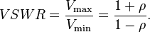
As ρ, the magnitude of Γ, always falls in the range [0,1], the VSWR is always ≥ +1.
The SWR can also be defined as the ratio of the maximum amplitude of the electric field strength to its minimum amplitude, i.e. Emax / Emin.
Further analysis
To understand the standing wave ratio in detail, we need to calculate the voltage (or, equivalently, the electrical field strength) at any point along the transmission line at any moment in time. We can begin with the forward wave, whose voltage as a function of time t and of distance x along the transmission line is:


This form of the equation shows, if we ignore some of the details, that the maximum voltage over time Vmot at a distance x from the transmitter is the periodic function


Standing wave ratio for a range of ρ. In this graph, A and k are set to unity.
Practical implications of SWR
The most common case for measuring and examining SWR is when installing and tuning transmitting antennas. When a transmitter is connected to an antenna by a feed line, the impedance of the antenna and feed line must match exactly for maximum energy transfer from the feed line to the antenna to be possible. The impedance of the antenna varies based on many factors including: the antenna's natural resonance at the frequency being transmitted, the antenna's height above the ground, and the size of the conductors used to construct the antenna.[1]When an antenna and feedline do not have matching impedances, some of the electrical energy cannot be transferred from the feedline to the antenna.[2] Energy not transferred to the antenna is reflected back towards the transmitter.[3] It is the interaction of these reflected waves with forward waves which causes standing wave patterns.[2] Reflected power has three main implications in radio transmitters: Radio Frequency (RF) energy losses increase, distortion on transmitter due to reflected power from load[2] and damage to the transmitter can occur.[4]
Matching the impedance of the antenna to the impedance of the feed line is typically done using an antenna tuner. The tuner can be installed between the transmitter and the feed line, or between the feed line and the antenna. Both installation methods will allow the transmitter to operate at a low SWR, however if the tuner is installed at the transmitter, the feed line between the tuner and the antenna will still operate with a high SWR, causing additional RF energy to be lost through the feedline.
Many amateur radio operators believe any impedance mismatch is a serious matter.[1] However, this is not the case. Assuming the mismatch is within the operating limits of the transmitter, the radio operator needs only be concerned with the power loss in the transmission line. Power loss will increase as the SWR increases, however the increases are often less than many radio amateurs might assume. For example, a dipole antenna tuned to operate at 3.75MHz—the center of the 80 meter amateur radio band—will exhibit an SWR of about 6:1 at the edges of the band. However, if the antenna is fed with 250 feet of RG-8A coax, the loss due to standing waves is only 2.2dB.[2] Feed line loss typically increases with frequency, so VHF and above antennas must be matched closely to the feedline. The same 6:1 mismatch to 250 feet of RG-8A coax would incur 10.8dB of loss at 146MHz.[2]
--
Teone Salazar
Comunicaciones de RadioFrecuencia
http://en.wikipedia.org/wiki/Standing_wave_ratio
Suscribirse a:
Entradas (Atom)